Attention Mechanism and Transformer (Deep Learning Notes C5W4)
These are some notes for the Coursera Course on Sequence Models, which is the last part of the Deep Learning Specialization. This post is a summary of the course contents that I learned from Week 4.
These notes are far from original. All credits go to the course instructor Andrew Ng and his team.
Attention Mechanism
We have introduced the encoder-decoder architecture for tasks like machine translation, and it works quite well with short sentences. But researchers found that as the length of the sequence increases, model performance metrics like the BLEU score decreases significantly. This motivates a modification of such architecture called the attention model.
The idea of the attention mechanism is to use the output vectors of all the words in the sequence instead of just using the output vector of the last word. At a particular time step \(t\), the network may determine which words are important for this output position and only use the information from those words, i.e., pay attention to only those parts of the input sequence, to predict the output vector.
The way to do this is to first take all the activations from a pre-attention RNN corresponding to the input sequence, and aggregate them into a single context vector of fixed length. At each time step, we feed this context vector into a post-attention RNN to predict the output vector. This is illustrated by the diagram shown below.

The next diagram illustrates with further details how each one of the vectors \(\text{context}^{\langle t \rangle}\) is computed:

The one-step attention context is computed as a weighted sum of the pre-attention activations:
\[\text{context}^{\langle t \rangle} = \sum_{t'=1}^{T_x} \alpha^{\langle t, t' \rangle} \mathbf{a}^{\langle t' \rangle}\]where in this formula:
- \(\alpha^{\langle t, t' \rangle}\) are the attention weights representing the amount of attention that \(\hat{y}^{\langle t \rangle}\) should be paying to the activation \(\mathbf{a}^{\langle t' \rangle}\)
- each activation \(\mathbf{a}^{\langle t' \rangle}\) corresponds to a specific input word can contain a forward component and a backward component if we use a bidirectional pre-attention RNN, that is: \(\mathbf{a}^{\langle t \rangle} = [\overrightarrow{\mathbf{a}}^{\langle t \rangle}, \overleftarrow{\mathbf{a}}^{\langle t \rangle}]\)
The attention weights are computed with a SoftMax layer as:
\[\alpha^{\langle t, t' \rangle} = \frac{\mathrm{e}^{e^{\langle t, t' \rangle}}}{\sum_{t'=1}^{T_x} \mathrm{e}^{e^{\langle t, t' \rangle}}}\]where \(e^{\langle t, t' \rangle}\) are the energies, which are computed with a simple neural network (typically a small feed forward network, sometimes just a single-layer with a \(\tanh\) function as the activation). This network takes the hidden state of the post-attention RNN from the previous time step, \(\mathbf{s}^{\langle t-1 \rangle}\) (also called a repeat vector), together with the current activations of the pre-attention RNN, to output \(e^{\langle t, t' \rangle}\). Note that the computations for the energy variables are not explicitly shown.
The Transformer Architecture: A First Look
Fundamentally, the machine translation models that we have been studying so far operate on the principle of sequential computation, i.e., the computation of the most probable next word at each time step in these traditional RNN depend on the previous computations. As a consequence, such models do not well handle very long-range dependencies as early tokens must propagate through many hidden states without degrading before they could influence later outputs. Also, the sequential nature of traditional RNN makes parallelization essentially impossible.
Stemmed from these limitations, the transformer architecture was designed to solve such sequential tasks more efficiently and more effectively by using a self-attention mechanism. Transformer was first introduced in the famous paper “Attention is All You Need” in 2017 and has revolutionized the approach to text-generative models. Transformers are also applied in image recognition tasks, protein structure predictions, audio generation and many other domains. The use of self-attention paired with traditional convolutional networks allows for parallelization which greatly speeds up training.
The overall architecture of the Transformer is shown below.
The transformer model consists of two main blocks: the encoder and the decoder.
The encoder is responsible for making sense of the input. It reads the input sequence and creates a representation of the input that contains a complete understanding of the meaning of the input sequence. Lying at the core of the encoder is the multi-head self-attention mechanism, which allows every word to interact with every other word in the input, so that relationships and dependencies are understood.
The decoder then generates the output sequence, one word at a time. The decoder uses a masked self-attention mechanism, so that it only looks at the previously generated outputs but not the future ones, and then uses a multi-head cross attention to focus on relevant parts of the encoder’s representation to generate the next output.
There is yet one further important ingredient of the architecture, positional encoding, which allows the model to keep track of the relative order of words in the input sequence. Although positional encoding is applied at early stages for both encoder and decoder, we would talk about that later. Let’s first look at the most important mechanism of the transformer architecture, self-attention.
Self-Attention
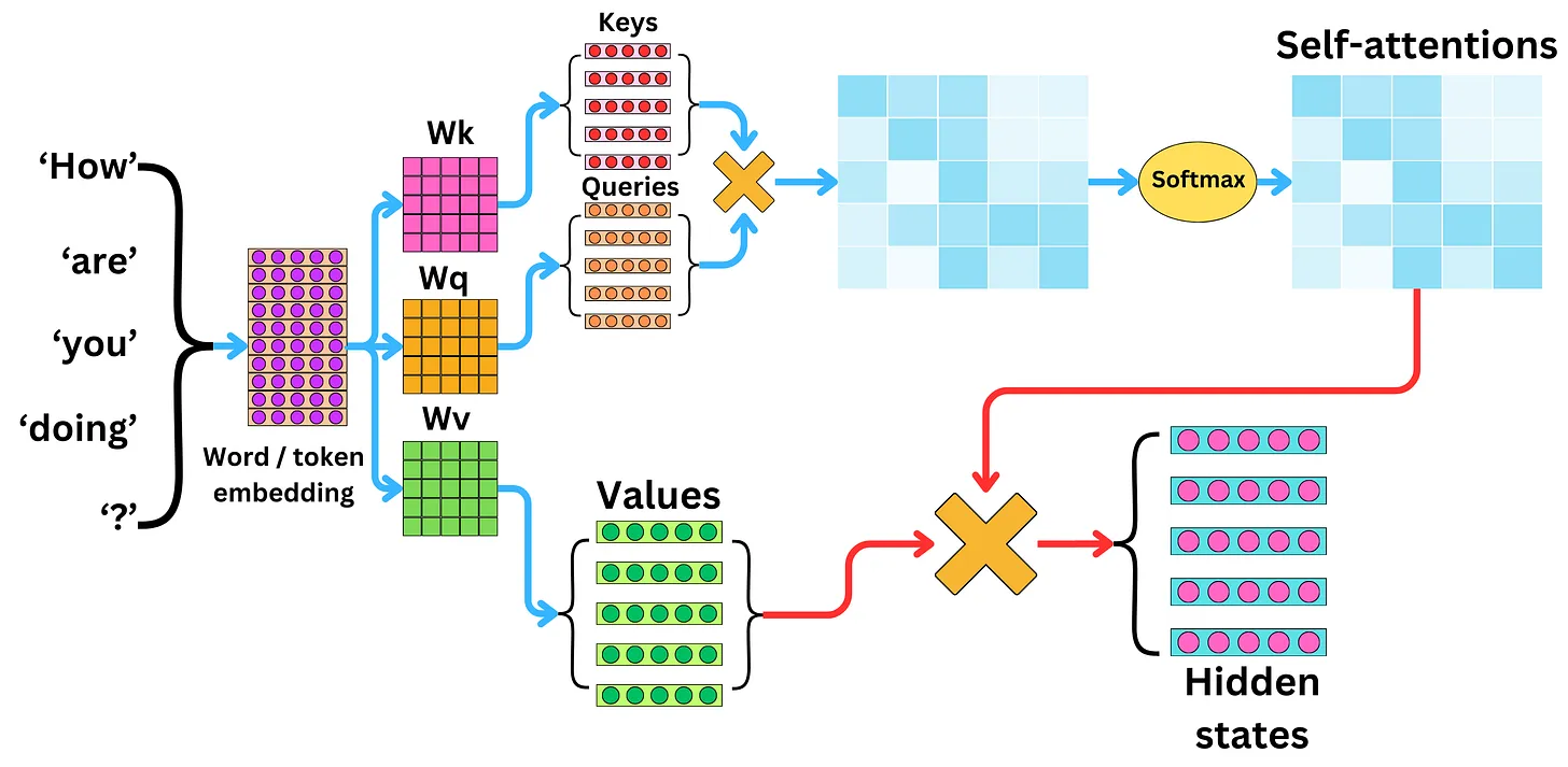
The self-attention is basically a scaled dot product attention, which takes in a query \(\mathbf{q}\), a key \(\mathbf{k}\) and a value \(\mathbf{v}\) as inputs to return attention-based vector representations of the words in the input sequence.

This can be mathematically expressed as:
\[\text {Attention}(Q, K, V)=\text{softmax}\left(\frac{Q K^{T}}{\sqrt{d_{k}}}\right) V\]- \(Q\) is the matrix of queries
- \(K\) is the matrix of keys
- \(V\) is the matrix of values
- \({d_k}\) is the dimension of the keys, and division by \(\sqrt{d_k}\) is used to scale everything down so that the SoftMax does not explode
Intuitively, we can think of the role of \(\mathbf{q}\), the query, as asking the question: for the current input word, what is the most relevant thing to search for? Then we check that with \(\mathbf{k}\)’s, the keys of every other word, to see which words are worth paying more attention to (greater values of the dot product \(\mathbf{q}\cdot\mathbf{k}\) means stronger relationship). Such words would return a vector \(\mathbf{v}\) with which we can finally take a weighted sum to compute the attention vector.
This process is very much like how we find a desired book in a library. Suppose we want to get a book on hardcore science so we ask whether there is anything to read on theoretical physics (that is the query). We then skim through the catalogue with the book titles and introductions like The Lord of the Rings, Hamlet or Quantum Field Theory (these are the keys), and we find that Quantum Field Theory is the best match, so we get that textbook and read the contents (that is the value).
Note that with self-attention, all positions are processed simultaneously, enabling parallelization over the input sequence. Also, any two positions in the sequence can interact directly regardless of how far apart they are, whereas traditional RNNs require multiple sequential steps. That allows the transformer model to retain long-range dependencies better.
Multi-Head Attention
Multi-head attention extends the self-attention mechanism by applying self-attentions for multiple times in parallel, so that each head can focus on different aspects of the input data. This allows the model to capture more complex relationships between words from different perspectives. The outputs of the multiple heads are then concatenated to produce the output.
Mathematically, multi-head attention is computed as a linear transformation of the concatenated representation via learnable parameters \(W_o\) by:
\[\text {MultiHead}(Q, K, V)=\text{Concat}\left( \text{head}_1, \text{head}_2, \cdots, \text{head}_h \right) W_o\]where attention vector of each head is:
\[\text{head}_i = \text {Attention}({W_i}^Q Q , {W_i}^K K, {W_i}^V V)\]Here, \({W_i}^Q\), \({W_i}^K\) and \({W_i}^V\) are learnable matrices for the \(i\)-th head. These projection matrices are introduced to reduce the dimensionality of the hidden states for faster training.
The following diagrams beautifully summarise the computation of a single-head self-attention and the multi-head self-attention.

Masked Self-Attention
There are two types of useful masks twhen building the Transformer network: the padding mask and the look-ahead mask.
To have uniform length for input sequences, those sequences longer than the maximum length would be truncated and zeroes are added to sequences shorter than the maximum length. However, these zeros will affect the SoftMax calculation. This is when a padding mask comes in handy. One approach is to define a mask that sets all the zeros in the sequence to a value close to negative infinity, so that the zeroes do not affect the score when we take the SoftMax.
The look-ahead mask follows a similar intuition. In training, we have access to the entire correct output sequence of the training example. The look-ahead mask prevents the model from cheating by looking ahead, ensuring it only makes prediction on the next output based on past and current tokens. This can be done similarly by masking out the future tokens with values close to negative infinity.
Positional Encoding
While self-attention mechanism is able to capture relationships between words from a global perspective, it does not preserve the relative order of the words which are also extremely important in sequential tasks.
Positional encoding is a standard approach to reintroduce positional information into embedding vectors. The sum of the positional encoding and word embedding is ultimately what is fed into the model. Here are the positional encoding equations we use for the transformer architecture:
\[\text{PE}(p, k) = \left\{ \begin{array}{ll} \displaystyle \text{PE}(p, 2i) = \sin\left(\frac{p}{10000^{\frac{2i}{d}}}\right) & \text{if } k=2i\\ \displaystyle \text{PE}(p, 2i+1) = \cos\left(\frac{p}{10000^{\frac{2i}{d}}}\right) & \text{if } k=2i+1 \end{array}\right.\]where
- \(p\) is the position of the word in the sequence (i.e., the first word in the sentence has \(p=0\), the second word has \(p=1\), and so on)
- \(k\) refer to the component of the positional encoding vector with \(i=k//2\), and by convention we use sine for even components and cosine for odd components
- \(d\) is the dimension of the word embedding and positional encoding
The following plot shows the heatmap for positional encodings with \(d=100\).

To develop some intuition about positional encodings, we can think of them broadly as a feature that contains the information about the relative positions of words. Word embeddings get enriched with positional information with the positional encoding being added in, but they are not significantly distorted as the values of the sines and cosines are small numbers.
Notice some interesting properties of the matrix. The first is that the norm of each of the vectors is always a constant. Let’s assume that \(d\) is even, then for any value of \(p\), we have
\[\begin{align*} \lVert \text{PE}(p) \rVert^2 &= \sum_{k=0}^{d-1} \left(\text{PE}(p,k)\right)^2 \\ &= \sum_{i=0}^{\frac{d}{2}-1} \left[ \sin^2 \left(\frac{p}{10000^{\frac{2i}{d}}}\right) + \cos^2 \left(\frac{p}{10000^{\frac{2i}{d}}}\right) \right] \\ \Rightarrow \lVert \text{PE}(p) \rVert^2 &= \frac{d}{2} \end{align*}\]which shows that the norm of the positional encoding would always be the same value. Hence, the dot product of two positional encoding vectors is not affected by the scale of the vector, which has important implications for correlation calculations.
We can also consider the norm of the difference between two positional encoding vectors separated by \(r\) positions is also constant if we keep \(r\) fixed:
\[\begin{align*} \lVert \text{PE}(p+r) - \text{PE}(p) \rVert^2 &= \sum_{k=0}^{d-1} \left(\text{PE}(p+r,k) - \text{PE}(p,k)\right)^2 \\ &= \sum_{i=0}^{\frac{d}{2}-1} \left\{ \left[ \sin \left(\frac{p+r}{10000^{\frac{2i}{d}}}\right) - \sin \left(\frac{p}{10000^{\frac{2i}{d}}}\right) \right]^2 + \left[ \cos \left(\frac{p+r}{10000^{\frac{2i}{d}}}\right) - \cos \left(\frac{p}{10000^{\frac{2i}{d}}}\right) \right]^2 \right\}\\ &= \sum_{i=0}^{\frac{d}{2}-1} \left\{ 2 - 2 \sin \left(\frac{p+r}{10000^{\frac{2i}{d}}}\right) \sin \left(\frac{p}{10000^{\frac{2i}{d}}}\right) - 2 \cos \left(\frac{p+r}{10000^{\frac{2i}{d}}}\right) \cos \left(\frac{p}{10000^{\frac{2i}{d}}}\right) \right\} \\ &= \sum_{i=0}^{\frac{d}{2}-1} \left\{ 2 - 2 \cos \left(\frac{p+r}{10000^{\frac{2i}{d}}}- \frac{p}{10000^{\frac{2i}{d}}}\right) \right\} \\ &= \sum_{i=0}^{\frac{d}{2}-1} \left\{ 2 - 2 \cos \left(\frac{r}{10000^{\frac{2i}{d}}}\right) \right\} \\ \Rightarrow \lVert \text{PE}(p+r) - \text{PE}(p) \rVert^2 &= d - 2\sum_{i=0}^{\frac{d}{2}-1} \cos \left(\frac{r}{10000^{\frac{2i}{d}}}\right) \end{align*}\]This shows that the difference between two positional encoding vectors separated by a fixed distance has a norm does not depend on the absolute positions of each encoding, but depends on the relative separation only. We can further show that we can shift the position \(p\) by any fixed offset \(r\) with a linear transformation (something very similar to a rotational matrix) that is independent of \(p\), i.e., it is possible to express the positional encoding at position \(p+r\) as linear function of the positional encoding at position \(p\). This makes it easier for the self-attention mechanism to learn and rely on relative distances, such as two words before or three words after.
Other Crucial Components in the Transformer Model
Feed Forward Network (FFN)
There is another important component located after the multi-head attention within both the encoder and decoder blocks known as the feed forward network (FFN). It acts as a position-wise processing unit that refines the representations after attention. By applying ReLu or GELU as activation functions, FFN introduces non-linearity into the model so complex non-linear relationships can be learned. FFN is also position-wise independent, meaning that the same transformation is applied to every token independently, so the computations can be done in parallel, which makes the model highly efficient.
Residual Connections and Layer Normalization
Each layer within the encoder and decoder blocks - whether a multi-head attention layer or a feed forward network - is wrapped with two additional supporting operations: a residual connection followed by layer normalization.
The residual connection adds the sub-layer’s input directly to its output before passing the result forward. This technique was originally introduced in ResNets for image recognition to address the vanishing gradient problem, and the transformer architecture borrows it directly. These shortcut connection highways allow gradients to flow directly across layers, mitigating vanishing gradients and enabling more stable convergence.
Layer normalization then normalizes the summed output across the feature dimension (zero mean and unit variance). This also stabilizes the hidden state activations throughout the network, preventing them from growing too large or collapsing to zero as the signal passes through many layers.
Together, residual connections and layer normalization make it practical to stack many encoder and decoder layers without the training process becoming unstable.
Transformers: Wrapping Up
Let’s finish this note by revisiting the transformer architecture.
- First the input sequence passes through an encoder that contains repeated encoder layers of
- embedding and positional encoding of the input
- multi-head attention on the input
- feed forward neural network to help detect features
- Then the predicted output passes through a decoder, consisting of the decoder layers of
- embedding and positional encoding of the output
- masked multi-head attention on the generated output
- multi-head cross attention with the \(Q\) from the masked multi-head attention layer and the \(K\) and \(V\) from the encoder
- a feed forward neural network to help detect features
- Finally, after the decoder layers, one dense layer and a SoftMax are applied to generate prediction for the next output in the sequence.